Estimating Phenolics from Spectra
Introduction
Since 2013, we have passed every must and wine sample through a spectrometer — daily through each fermentation, at every cellar sampling, and, in recent vintages, on the berries and juice before harvest. A companion note, Spectra and Color Evolution (Spectra and Color Evolution — Chateau Hetsakais), showed what those spectra say about color. This note goes a step further, from color to chemistry: it reviews how the spectra can estimate the phenolic compounds that actually build the wine — the anthocyanin pigments, the tannins, and the iron-reactive phenolics.
The conventional approach to measuring phenolic components is using the time-consuming and thus expensive Adams-Harbertson assay in a wet laboratory. The modern alternative is to use a service provider that has correlated an extensive database of Adams-Harbertson results with the spectra of the respective samples. The service bureau then uses these correlations to shortcut the wet laboratory by estimating the phenolic components of new samples based on their spectra alone. By keeping the correlations proprietary, the service provider can replace the high cost of the wet laboratory with the low cost of measuring the sample spectrum and computation. We have used WineXRay (WineXRay for Phenolics in Wine — Chateau Hetsakais) to provide this fee-based service since 2014. Substituting the expensive wet-lab analysis with WineXRay, or any of its competitors (TheWineCloud, CloudSpec, ETS Laboratories, etc), has drawbacks:
The estimation error of the wet-laboratory is compounded by the estimation error of the proprietary correlations used.
Our own spectrometer may produce slightly different measurements than the spectrometer used by the service provider for the base samples underlying the correlation, thus adding to the estimation error.
The integration of external service providers with our own systems, exporting spectra and receiving results, is manual and cumbersome, and prone to additional errors.
So far, we have tried to adjust the most egregious outliers after visual inspection manually. The following graphic illustrates the “error problem”. It shows, on the left, the estimated Bound Anthocyanins during the fermentation of Cabernet Sauvignon in 2013, as reported by WineXRay (WXBAnt, the “raw” data), vs. a trajectory of the data; and, on the right, the same with the manually adjusted data (WXBAntU, the “used” data).
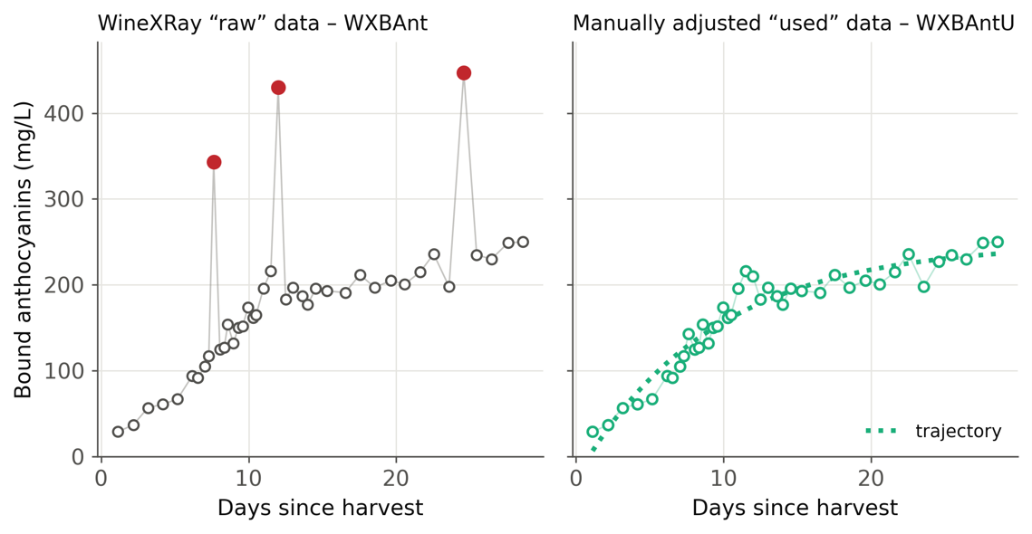
Figure 1. Bound anthocyanins over the 2013 Cabernet Sauvignon fermentation. Left: as reported by WineXRay (WXBAnt), with three spurious spikes (red). Right: after manual adjustment (WXBAntU), the spikes are pulled back onto the trajectory.
Clearly, there is significant noise here. Bound Anthocyanins are supposed to rise and fall smoothly – like the trajectory – but they don't, and the sources of the errors are not clearly identifiable. We decided to address the drawbacks by fully internalizing the estimation process with the following approach:
We use our own history of over 2,000 spectra, collected WineXRay estimates, and underlying chemical and colorimetric data to estimate our "correlation". Using our own history most probably increases the estimation errors
We adjust the initial results of our own "correlation" using trajectories estimated for each berry, fermentation, or cellar batch over its life. The use of trajectories should reduce the estimation errors.
By taking the process fully in-house, we eliminate possible errors from data transfer and differences in spectrometer measurements.
The idea of describing a phenolic's path over the life of a batch with a smooth curve is not itself new: a substantial literature models the extraction and evolution of color and phenolics through red-wine maceration and aging, and reviews of that work catalog the empirical and mechanistic curve families used to do so [8], [9]. What is novel here is the purpose we put those trajectories to. Rather than fitting a curve to describe the underlying chemistry, we use trajectories as a second layer on top of the spectral estimates — first to clean the data, by rejecting readings that stray from a batch's own smooth path, and then to validate and retroactively adjust the single-spectrum estimates against the trajectory drawn through them. Coupling an instantaneous, spectrum-by-spectrum estimate to the temporal path of the batch it belongs to is the heart of our approach.
Here is a preview of the results. The side-by-side graphic compares WineXRay's estimates for the same example shown above with our internal results.
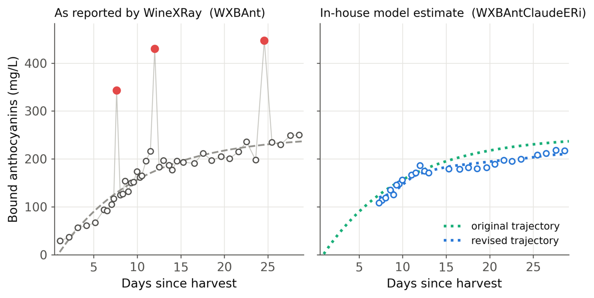
Figure 2. The same fermentation. Left: WineXRay as reported (WXBAnt), with the three spikes (red). Right: our in-house model estimate (WXBAntClaudeERi, circles), which is free of the artifacts. Two reference curves are shown: a trajectory fit to the raw data (green) and the revised trajectory (blue, WXBAntClaudeERiTraj) fit through the model estimates; the two run close together. Estimates begin on day 7, when filtered spectra are available.
This note explains our new estimation process in detail.
Step 1 - Filtered Spectra & Color Parameters: We start by filtering out noise from all our spectral measurements and computing color parameters for each spectrum.
Step 2 - Recorded Phenolics and their Estimated Trajectories: We examine how recorded phenolics evolve over the life of a berry lot, a fermentation, and a cellar batch, and fit a smooth trajectory to each.
Step 3 – Adjusting for outliers: We fit each phenolic's trajectory to the raw WineXRay values, flag any reading more than 2 standard deviations off that first-pass curve, drop the flagged points, and refit — a two-pass robust fit.
Step 4 – Estimating Phenolics from a single Spectrum: We build models that estimate phenolics directly from a single spectrum using past observations, but we only include instances that are not flagged as outliers by the 2-standard-deviation trajectory rule.
Step 5 - Trajectory of Estimated Phenolics: We push those estimates back through the trajectory fitter, check that the estimated path matches the recorded one, and adjust the model retroactively to the respective berry, fermentation, or cellar batch.
Step 6 – Understanding Interventions: We ask whether and how interventions such as acid, carbonate, sulfur, fining, barrel changes — leave a mark on the phenolics.
Step 7: Spreadsheet Implementation: Finally, we fold the whole chain into a spreadsheet a cellar hand can use the moment a spectrum comes off the instrument
We close with a section on what we learned and where this may lead to next (8).
Step1: Filtered Spectra and Color Parameters
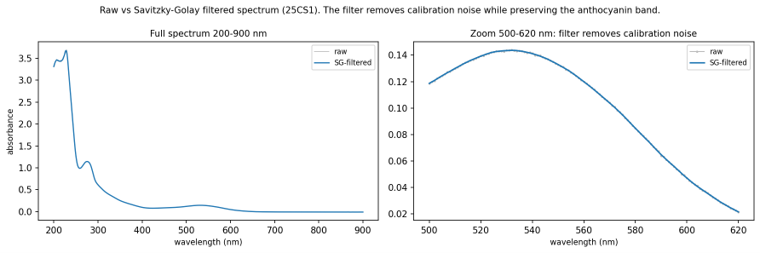
Another page on the website describes in detail how we filter out measurement noise from the spectrometer and compute industry-standard colorimetric parameters (Spectra and Color Evolution — Chateau Hetsakais). Every time we touch the must or wine, we measure and record an absorbance curve, sampled at 1 nanometer intervals from 200 to 900 nm. Raw absorbance carries symmetric measurement noise from re-zeroing the instrument against distilled water. So before anything else, we smooth each curve with an eleven-point, second-order Savitzky–Golay filter and compute the industry-standard CIE L*a*b* color parameters. While we provide the unfiltered spectra to WineXRay as input for their phenolic estimation, we use only filtered data in our analysis. The following graphic shows the minute impact of filtration.